Fourier,neural,operator,approach,to,large,eddy,simulation,of,three-dimensional,turbulence

Zhijie Li, Wenhui Peng,d, Zelong Yuan, Jianchun Wang,*

a Department of Mechanics and Aerospace Engineering, Southern University of Science and Technology, Shenzhen 518055, China

b Southern Marine Science and Engineering Guangdong Laboratory (Guangzhou), 511458, China

c Guangdong-Hong Kong-Macao Joint Laboratory for Data-Driven Fluid Mechanics and Engineering Applications, Southern University of Science and Technology, Shenzhen 518055, China

d Department of Computer Engineering, Polytechnique Montreal, Montreal H3T1J4, Canada

Keywords:Fourier neural operator Large eddy simulation Data-driven simulation Incompressible turbulence

ABSTRACT Fourier neural operator (FNO) model is developed for large eddy simulation (LES) of three-dimensional(3D) turbulence. Velocity fields of isotropic turbulence generated by direct numerical simulation (DNS)are used for training the FNO model to predict the filtered velocity field at a given time. The input of the FNO model is the filtered velocity fields at the previous several time-nodes with large time lag. In the a posteriori study of LES, the FNO model performs better than the dynamic Smagorinsky model (DSM)and the dynamic mixed model (DMM) in the prediction of the velocity spectrum, probability density functions (PDFs) of vorticity and velocity increments, and the instantaneous flow structures. Moreover,the proposed model can significantly reduce the computational cost, and can be well generalized to LES of turbulence at higher Taylor-Reynolds numbers.

In recent years, data-driven approaches based on machine learning (ML) have been widely used to accelerate computational fluid dynamics (CFD) [1,2]. These studies can be mainly classified as ML-assisted modeling approaches which aim to fit the unclosed term of classical turbulence models [3–7], and pure data-driven approaches which aim to approximate the Navier-Stokes equations directly by deep learning methods [8,9]. Ling et al. [10] used a deep learning method to predict the Reynolds stress tensor with the Galilean invariance. Beck et al. [11] presented a method of using the convolution neural network (CNN) and residual neural network (RNN) to build more accurate large eddy simulation (LES)models. Park and Choi [12] developed a subgrid-scale (SGS) model using a fully connected neural network in LES of channel turbulence. Wang et al. [13] proposed a semi-explicit deep learning framework to reconstruct the SGS stress in LES of incompressible turbulence.

Although ML-assisted modeling approaches have the potential to achieve more accurate results than classical turbulence models,it is still hard to significantly reduce the computational cost. In contrast, the pure data-driven methods, like a “black-box” model,can make predictions very quickly and efficiently compared with traditional methods [14–16]. Han et al. [17] proposed a hybrid deep neural network model to learn the spatial-temporal features of the unsteady flow fields. Ren et al. [18] combined the long short-term memory and convolution neural network to predict the temporal evolution in turbulence. Guan et al. [19] used a deep convolutional neural network and transfer learning to improve the accuracy and stability of the prediction in turbulence. Li et al. [20] proposed a Fourier neural operator (FNO) framework which can directly learn the mapping between infinite dimensional spaces from a series of input-output pairs. The FNO can perform better than the state-of-the-art models in two-dimensional turbulence prediction tasks on account of its efficient and expressive architecture. Peng et al. [21] introduced an attention-enhanced FNO model which can accurately reconstruct various statistical properties and instantaneous flow structures of two-dimensional (2D) turbulence at high Reynolds numbers. In recent years, FNO has received more and more attention, but it has not been used in the study of threedimensional (3D) turbulence.

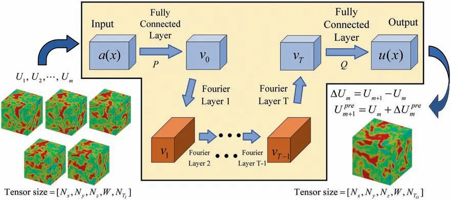
Fig. 1. Architecture of the Fourier neural operator (FNO) for 3D turbulence prediction. Note that the black box shows the FNO architecture, the lower left corner shows the input of the model, and the lower right corner shows the result calculated from the model output. Here, Nx =Ny =Nz =32 denotes grid resolutions, W =3 is number of dimensions, NTI =5 and NTO =1 are the numbers of time-nodes. T = 4 is the number of Fourier layer and each layer contain 20 Fourier modes, m=5.

In this paper, we apply the FNO approach to LES of threedimensional turbulence. We take the filtered velocity fields at previous several time-nodes as inputs of the FNO model and expect that the FNO model can learn the evolution of turbulence from the dataset. It is shown that the FNO model can perform with a higher accuracy, more efficiency, and good generalization ability in comparison with traditional SGS models in thea posterioristudies of LES.

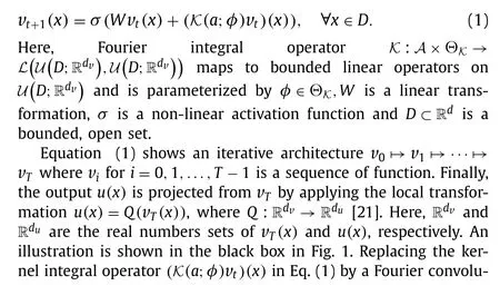
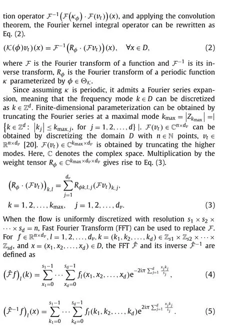
Most neural network methods are used to learn the mapping between finite-dimensional Euclidean spaces. They can perform well for particular governing equations but are difficult to generalize when the parameters of the equations or conditions change[22–24]. The Fourier neural operator learns the mapping relationships between infinite dimensional spaces from a series of inputoutput pairs, meaning that FNO learns the rule of an entire family of PDE by using data-driven methods [20]. The FNO model converts the convolution operation in the neural network into a multiplication operation through discrete Fourier transform, which can greatly improve the computational efficiency.

Denote the target non-linear map asG†:A→UwhereA=AD;RdaandU=UD;Rduare separable Banach spaces of function taking values in Rdaand Rdu, respectively [25]. HereD⊂Rdis a bounded, open set. R is real number space, and Rdaand Rduare the values sets ofa(x)andu(x), respectively. Here,da,duanddvis the dimensions of inputa(x), outputu(x)andvT(x), respectively. By constructing a parametric mapG:A×Θ→U, the Fourier neural operators can learn to approximateG†. By using data-driven methods, FNO will adjust the optimal parameterθ†∈Θso thatG·,θ†=Gθ†≈G†. The inputa(x)is first transformed to a higher dimensional representationv0(x)=P(a(x))by a shallow fully-connected layerP. Thenv0(x)is updated iteratively by Eq. (1),

A filtering technique can be introduced to separate the physical quantities in turbulence into resolved large-scale and sub-filter small-scale quantities [26,27]. For any fieldsfin Fourier space, a filtered field is defined as ¯f(k)= ˆG(k)f(k). In this study, the sharp spectral filter is used in Fourier space which is defined as ˆG(k)=H(kc−|k|), Here, cutoff wavenumberkc=π/l, andldenotes the filter width. The Heaviside step functionH(x)=1 ifx≥0; other-wiseH(x)=0 [28]. The filtered incompressible Navier-Stokes equations for the resolved fields can be rewritten as [27,29]

Table 1 Parameters of the 3D FNO model.

The direct numerical simulation (DNS) is performed with the grid resolutions of 2563at the Taylor Reynolds numberReλ≈100.The DNS data is filtered into large-scale flow fields at grid resolutions of 323by the sharp spectral filter with cutoff wavenumberkc=10. The advanced time step is set to be 10−3and the numerical solution is recorded every 200 steps as a time-node. In this numerical simulation, 45 groups of different random fields are used as the initial fields for subsequent calculations and 600 time-nodes for each group of calculations are stored. Here, we stored the DNS data after the flow fields become statistically steady. The filtered direct numerical simulation (fDNS) data of size 45×600×32×32×32×3 can be obtained as the training and testing dataset,which contains 45 groups, each group has 600 time-nodes, and each time-node is a velocity field of 323with three directions. 595 input-output pairs of velocity fields can be generated from 600 time-nodes. Therefore, 45 groups contain a total of 26775 sample pairs of velocity fields, where 80% of the samples are used for training and 20% for testing.

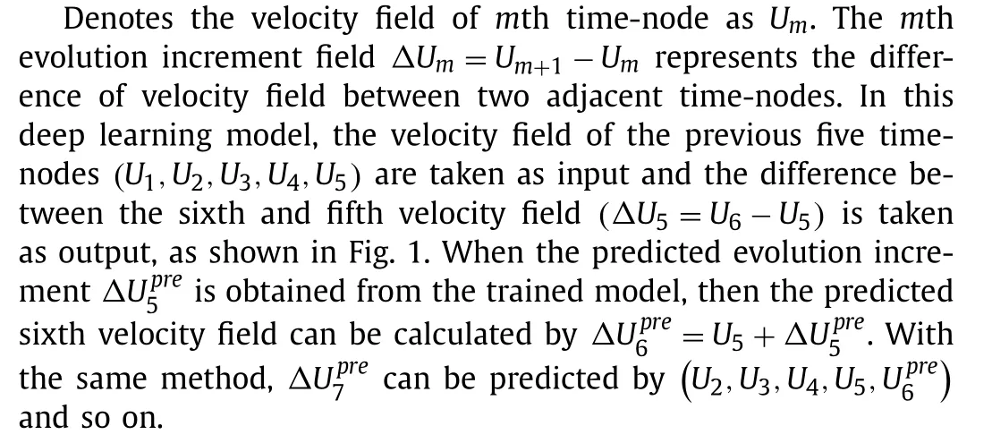
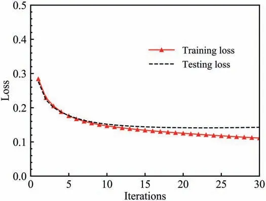
Fig. 2. Learning curves of the FNO model for LES of 3D turbulence.

The parameters of the 3D FNO model are listed in Table 1. In the process of optimizing the number of modes and the number of Fourier layers, we found that when choosing 4 Fourier layers with 20 modes for each layer, the model performance is better.When the numbers of Fourier layers and modes are set to large values, it will lead to too many model parameters and the calculation consumption is too large. When the numbers of Fourier layers and modes are small, the model accuracy will be insufficient. The ReLU function and adaptive moment estimation (Adam) are chosen as the activation function and optimizer, respectively [34]. The FNO model is trained for 30 epochs with a learning rate of 0.0001 and batch size of 2. The learning curves of the FNO model for LES of 3D turbulence are shown in Fig. 2. It can be seen that the curves of training loss and testing loss are well convergent and quite close to each other.

To ensure the generalization of the model, five more groups of data from different initial fields are generated and used for thea posterioritest. In the followinga posterioritest, the FNO model compares with the results from fDNS data and classical LES models, including the dynamic Smagorinsky model (DSM) and the dynamic mixed model (DMM) [35–37]. All simulations are initialized by the same flow field of filtered DNS data. The spectra of velocity and velocity error field (error compared with fDNS data) at fifteenth time-nodes(t/τ=4.29)are shown in Fig. 3.Hereτ≡LI/urmsdenotes the large-eddy turnover time [38] and is about 0.7.LIdenotes the integral scale andurmsis the rootmean-square (RMS) of velocity. The interval between every two adjacent time-nodes isΔt=0.2 and the dimensionless time isΔt/τ=0.286. For different models, the errors of the velocity spectrum increase askincreases. Both classical LES models can agree well with fDNS in the low-wave number region and deviate significantly from fDNS near the cut-off wavenumber. In contrast,the FNO model can well reconstruct the velocity spectrum at different flow scales. Meanwhile, the spectra of the velocity error field predicted by FNO are less than those predicted by DSM and DMM near the cut-off wavenumber region. Therefore, the velocity spectrum predicted by the FNO model is very close to that of fDNS.

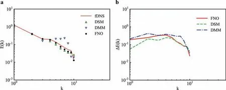
Fig. 3. Spectra of velocity and velocity error field for LES at t/τ =4.29: a velocity spectrum, b velocity error field spectrum.

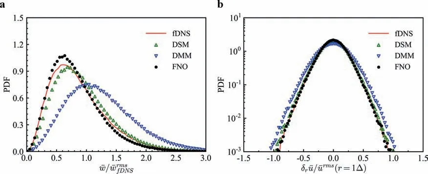
Fig. 4. PDFs of normalized vorticity and normalized increments of the velocity for LES at t/τ =4.29: a normalized vorticity, b normalized increments of the velocity.

Figure 4 shows the probability density functions (PDFs) of the normalized vorticity and the normalized velocity incrementδr¯u/¯urms, whereδr¯u=[¯u(x+r)−¯u(x)]·ˆr represents the longitudinal increment of the velocity at the separation r. Here, ˆr=r/|r|.The vorticity and the velocity increment are normalized by the RMS values of vorticity ¯ωrmsand velocity ¯urms, respectively. It can be seen that both FNO and DSM models can predict the PDF of¯ω/¯ωrmsbetter than that of the DMM model, and the prediction by FNO model is closer to that of fDNS than DSM model for ¯ω/¯ωrmsless than 0.5 and between 0.8 to 1.5. which indicates that the FNO model can reconstruct the vortical coherent structures more accurately in this case. The PDF ofδr¯u/¯urmspredicted by the DMM model is significantly wider than that of fDNS. In contrast, the PDFs predicted by the FNO and DSM models are in good agreement with that of fDNS.

The spatial structures of vorticity of fDNS and LES with DSM and FNO models at the instantt/τ≈1.0 (third time-node) are shown in Fig. 5. It can be seen that the large vortex structures from fDNS can be caught by both DSM and FNO models. Moreover, the overall instantaneous vorticity structures predicted by FNO model are much closer to those of fDNS, as compared to those of DSM model.

Figure 6 illustrates the comparison of the predictions of velocity spectrum and PDFs of normalized vorticity at different timet/τ. It can be seen that the velocity spectrum and PDFs of normalized vorticity predicted by FNO model are significantly better than those of DSM and DMM models att/τ≈1.0. As time increases,the error of velocity spectrum predicted by different models will increase. However, the velocity spectrum predicted by FNO is still better than those of DSM and DMM models att/τ≈5.71. The PDFs of normalized vorticity predicted by FNO and DSM models have a good agreement with fDNS att/τ≈5.71.

Moreover, the generalization ability of the 3D FNO model is tested. The well-trained FNO model can be directly used to predict the fDNS data at higher Taylor Reynolds numbers. Figure 7 compares the velocity spectrum and PDFs of normalized vorticity of isotropic turbulence at Taylor Reynolds numbersReλ≈160 andReλ≈250, respectively. It can be seen that the PDFs of normalized vorticity predicted by DSM and DMM models have large discrepancy with that of fDNS. Because the computational grid is very coarse, the dissipation of the traditional model is insufficient at high Taylor Reynolds numbers. In the Fig. 7, the legend named‘DSM G64’and ‘DMM G64’denote the results of DSM and DMM models computed with a resolution of 643grids. It can be seen that increasing the number of grids can improve the performance of the DSM and DMM models, but they are still slightly worse than the FNO model in terms of velocity spectrum and PDFs of normalized vorticity. However, in the case of low Taylor Reynolds numbers, due to the large physical viscosity, better results can also be obtained by traditional models. In contrast, the velocity spectrum and PDFs of normalized vorticity predicted by the FNO model are in good agreement with fDNS at high Taylor Reynolds numbers,which are significantly better than those of DSM and DMM models. Since turbulent flow data for high Taylor Reynolds numbers are not readily available in many situations, it is important to train the FNO model using data with lower Reynolds numbers and apply the well trained model to turbulence at high Taylor Reynolds numbers.Considering the self-similarity of turbulence, the large-scale statistical features and flow structures in some regions are insensitive to the Taylor Reynolds numbers, which provides a theoretical basis for developing such a model.

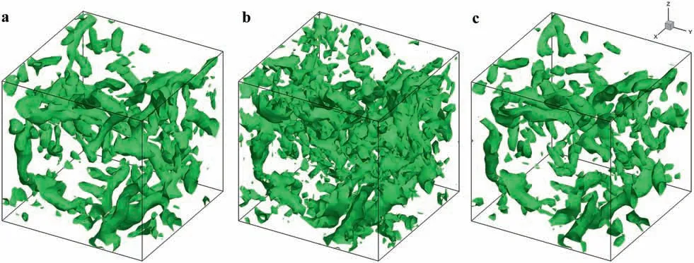
Fig. 5. Isosurface of the normalized vorticity ω¯/=1.5 at t/τ ≈1.0: a fDNS, b DSM, c FNO.

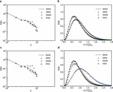
Fig. 6. Velocity spectrum and PDFs of normalized vorticity at different t/τ: a Velocity spectrum at t/τ ≈1.0, b PDFs of normalized vorticity at t/τ ≈1.0, c Velocity spectrum at t/τ ≈5.71, d PDFs of normalized vorticity at t/τ ≈5.71.

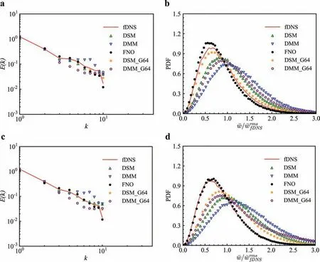
Fig. 7. Velocity spectrum and PDFs of normalized vorticity with different Taylor Reynolds numbers at t/τ =4.29 : a Velocity spectrum at Reλ ≈160, b PDFs of normalized vorticity at Reλ ≈160, c Velocity spectrum at Reλ ≈250, d PDFs of normalized vorticity at Reλ ≈250. Specially, the DSM G64 and DMM G64 represent the results computed with a resolution of 643 grids.

Another great advantage of the FNO model is its computational efficiency. The FNO model is trained on the Pytorch and MindSpore open-source deep learning frameworks. The DSM and DMM simulations are implemented on a virtual machine where the type of CPU is Intel Xeon Gold 6148 CPU @2.40 GHz. Using 32 cores to parallel accelerate the computation, 0.204s and 0.271s are taken for calculating per time-node of DSM and DMM models, respectively.In contrast, the prediction of the FNO model only takes 0.0311s for the same tasks which are conducted on a GPU type of NVIDIA GeForce RTX 2080 Ti. It is worth noting that the DSM and DMM models with 643grids take 6.23s and 9.94s to calculate per timenode, respectively, which are 199 and 330 times slower than FNO model.

Different from the traditional neural network that learns the mappings between input and output in the physical space, the FNO model replaces the kernel integral operator with a convolution operator defined in Fourier space and converts it into a multiplication operation by using discrete fast Fourier transform (DFFT).Therefore, compared with the traditional convolutional neural network (CNN) and U-Net models, the FNO model can perform a higher computational efficiency and well capture the multi-scale flow structure of convection-diffusion [20].

The FNO model can directly predict the evolution process of the flow field with a large time step, indicating that this model has learned the integral of the dynamic equation in this time period. However, it cannot be achieved by traditional discrete methods based on differential equations, due to the strong nonlinearity of the dynamical evolution in such a time period. This also explains the advantage of the FNO model in terms of computational efficiency from another perspective.

In this research, we develop an FNO approach to large eddy simulation of three-dimensional turbulence. Filtered DNS flow fields of isotropic turbulence at different times are used for training FNO models. In thea posterioritest of LES, it is shown that FNO performs better than the DSM and DMM models in the prediction of velocity spectrum, instantaneous flow structures, and PDFs of vorticity and velocity increments. The present FNO model can be used to predict large scale dynamics of isotropic turbulence at higher Taylor Reynolds numbers. Moreover, the FNO model shows its great potential in terms of computational speed. Our future work aims to improve the generalization ability of the model by using local neural operators avoiding periodic condition, incorporating physical constraints, and hybridizing with transitional methods.

Declaration of Competing Interest

The authors declare that they have no known competing financial interests or personal relationships that could have appeared to influence the work reported in this paper.

Acknowledgments

This work was supported by the National Natural Science Foundation of China (Nos. 91952104, 92052301, 12172161, and 12161141017), by the National Numerical Windtunnel Project (No.NNW2019ZT1-A04), by the Shenzhen Science and Technology Program (No. KQTD20180411143441009), by Key Special Project for Introduced Talents Team of Southern Marine Science and Engineering Guangdong Laboratory (Guangzhou) (No. GML2019ZD0103), by CAAI-Huawei MindSpore open Fund, and by Department of Science and Technology of Guangdong Province (No. 2019B21203001).This work was also supported by Center for Computational Science and Engineering of Southern University of Science and Technology.